Renormalization Group in Machine Learning

I worked on project in 2023 fall.

Abstract

In the phase transition theory, the correlation length diverges to infinity at the critical point which leads to many physical phenomena. We can use the mean-field theory and renormalization group theory to analyze these phenomena. But actually, similar phenomena happen not only in the phase transition but in many natural complex systems. Moreover, in these complex systems, people often use statistics to build the mathematical model. The neural network framework is a kind of algorithm that can be applied to justify which categorical data an individual belongs to. This process is similar to using the renormalization group theory to compute which phases a system belongs to. Therefore, although the precise mathematical structure hasn’t been built yet, we believe that the neural network framework can be viewed as the renormalization group theory.

Neural Network

• Framework of Model

First, I use the neural network model as an example for the reason that it’s a highly abstract mathematical model so that it can be extended to other models more easily. The fundamental structure of a neural network framework has three parts, an input layer, several hidden layers, and an output layer. Which can be expressed as a figure below. 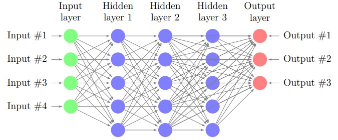This is a neural network having three hidden layers. Let four input signals be \(x_1, x_2, x_3\) , and \(x_4\) the first layer would output \(a^{[1]}_1,a^{[1]}_2,a^{[1]}_3,a^{[1]}_4,a^{[1]}_5\) to the second layer, the signals \(a^{[1]}_i\) are computed by the process below and with parameters weight : \(weight:\;W^{[1]}_{ij},\;bias:\;b^{[1]}_i\) and the activation function \(g\), where the index \([i]\) denotes the parameters for \(i^{th}\) hidden layer \(a^{[1]}_1=g(x_1 W^{[1]}_{11}+x_2 W^{[1]}_{21}+x_3 W^{[1]}_{31}+x_4 W^{[1]}_{41}+b^{[1]}_1)\\ a^{[1]}_2=g(x_1 W^{[1]}_{12}+x_2 W^{[1]}_{22}+x_3 W^{[1]}_{32}+x_4 W^{[1]}_{42}+b^{[1]}_2)\\ a^{[1]}_3=g(x_1 W^{[1]}_{13}+x_2 W^{[1]}_{23}+x_3 W^{[1]}_{33}+x_4 W^{[1]}_{43}+b^{[1]}_3)\\ a^{[1]}_4=g(x_1 W^{[1]}_{14}+x_2 W^{[1]}_{24}+x_3 W^{[1]}_{34}+x_4 W^{[1]}_{44}+b^{[1]}_4)\\ a^{[1]}_5=g(x_1 W^{[1]}_{15}+x_2 W^{[1]}_{25}+x_3 W^{[1]}_{35}+x_4 W^{[1]}_{45}+b^{[1]}_5)\) We can write parameters as matrices and vector \(\bf{W}^{[1]}=\begin{pmatrix} {W}^{[1]}_{11}&{W}^{[1]}_{12}&{W}^{[1]}_{13}&{W}^{[1]}_{14}&{W}^{[1]}_{15}\\ {W}^{[1]}_{21}&{W}^{[1]}_{22}&{W}^{[1]}_{23}&{W}^{[1]}_{24}&{W}^{[1]}_{25}\\ {W}^{[1]}_{31}&{W}^{[1]}_{32}&{W}^{[1]}_{33}&{W}^{[1]}_{34}&{W}^{[1]}_{35}\\ {W}^{[1]}_{41}&{W}^{[1]}_{42}&{W}^{[1]}_{43}&{W}^{[1]}_{44}&{W}^{[1]}_{45}\\ \end{pmatrix},\) \(\bm{x}=\begin{pmatrix} x_1\\ x_2\\ x_3\\ x_4 \end{pmatrix},\;\bm{a}^{[1]}=\begin{pmatrix} a_1^{[1]}\\ a_2^{[1]}\\ a_3^{[1]}\\ a_4^{[1]}\\ a_5^{[1]} \end{pmatrix},\;\bm{b}^{[1]}=\begin{pmatrix} b_1^{[1]}\\ b_2^{[1]}\\ b_3^{[1]}\\ b_4^{[1]}\\ b_5^{[1]} \end{pmatrix}\) then the computational process can be written as \(\bm{a}^{[1]}=g(\bf{x}\bf{W}^{[1]}+\bm{b}^{[1]}) \) Then, \(\bm{a}^{[1]}\) inputs to the second layer and output \(\bm{a}^{[2]}\), that is \(\bm{a}^{[2]}=g(\bm{a}^{[1]}\bf{W}^{[2]}+\bm{b}^{[2]})\) . Similarly, \(\bm{a}^{[2]}\) inputs to the second layer and output \(\bm{a}^{[3]}\), that is \(\bm{a}^{[3]}=g(\bm{a}^{[2]}\bf{W}^{[3]}+\bm{b}^{[3]})\) The final output is \(\bm{z}=g(\bm{a}^{[3]}\bf{W}^{[4]}+\bm{b}^{[4]})\) Generalize this process to any dimension of parameters and numbers of layers \(n\), it could be written as \(\bm{a}^{[i+1]}=g(\bm{a}^{[i]}\bf{W}^{[i+1]}+\bm{b}^{[i+1]})\) , where \(\bm{a}^{[0]}=\bm{x}\) and \(\bm{a}^{[n+1]}=\bm{z}\). There are many kinds of activation functions, in this report, I use \(g(\bm{z})=\frac{1}{\sum_je^{z_j}}\begin{pmatrix} e^{z_1}\\ e^{z_2}\\ \vdots\\ e^{z_n} \end{pmatrix}\) , where \(n\) is the dimension of the layer output.

• Training Model

We can see that if the parameters \(\{\bf{W}^{[k]},\bm{b}^{[k]}\}_k\) are all determined, then the model is determined, too. So now the question is how to determine the parameters, that is, how to train the model. If we have a training set, we can see parameters \(\{\bf{W}^{[k]},\bm{b}^{[k]}\}_k\) are the best ones if the prediction error is minimized. The prediction error can be defined as a loss function $\mathcal{L}$, this function is selected by the objects we want to predict. Here we select \(\mathcal{L}=cross\;entropy\) which is a function often used to justify the prediction error for categorical data. So now we only need to find which parameters \(\{\bf{W}^{[k]},\bm{b}^{[k]}\}_k\) minimizes \(\mathcal{L}\), this problem can be solved by many methods such as gradient descent method. In this report, we use the backward propagation method to train the model. Since the method used isn't associative with the topics, I do not discuss too much about it here.

Renormalization Group

I believe that the pruning of the neural network can be interpreted by the physical interpretation of the renormalization group. I would use some numerical experiments to explain this statement. I use the R language to build the neural network model, for it’s more convenient to see more statistical data and compute some statistical quantity

• Samples at the Critical Point

Recall that the renormalization group theory provides us a way to analyze the physical phenomena near the critical point, but actually, the concept of critical phenomena also appears in many natural systems. We use a numerical method to provide the critical phenomenon a statistics interpretation. I use a classical data set \(\bm{iris}\) in R as an example, we use the neural network to predict the categorical data \(\bm{Species}\). Before explaining the neural network is a kind of renormalization group, we need to explain what does critical point means for the samples in the data set. Let's visualize the predictors. First plot the scatter plots between the continuous predictors:


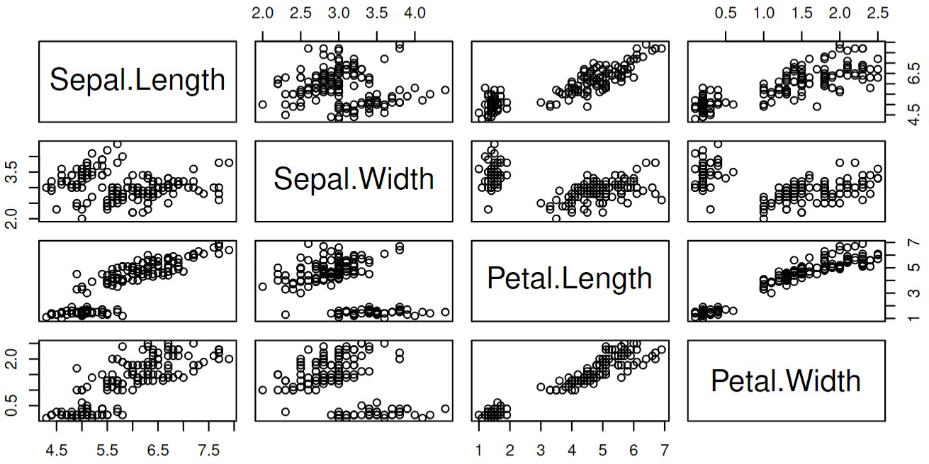
And compute the Pearson correlation between the continuous predictors:


Correlation matrix of the iris

	Sepal.Length	Sepal.Width	Petal.Length	Petal.Width
Sepal.Length	1.0000000	-0.1175698	0.8717538	0.8179411
Sepal.Width	-0.1175698	1.0000000	-0.4284401	-0.3661259
Petal.Length	0.8717538	-0.4284401	1.0000000	0.9628654
Petal.Width	0.8179411	-0.3661259	0.9628654	1.0000000


Since the response is a categorical variable, we draw the box plot to visualize its relation with other continuous predictors:


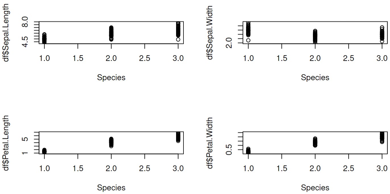
And compute the Point-Biserial correlation between the response and predictors:



Point-Biserial Correlation for iris

Sepal.Length	Sepal.Width	Petal.Length	Petal.Width
0.7825612	-0.4266576	0.9490347	0.9565473


We can see that some predictors have a significant correlation with the response. Moreover, some predictors have a significant correlation with other predictors, too. Considering there are 150 individuals in the data set and the randomness of sampling, we can believe that the parameters can have the predictors have such correlation in every individual. So we can say that even if sepals and petals are only small parts of the iris, they still highly correlate with other characters of the individuals. This is why we could say the samples are at a critical point. This phenomenon is why the biological systems have enough adapting ability. When the environment changes, the systems only need to change a little part of the biological character to adapt to the change. This is why many biological systems are at the so-called critical point.

• Neural Network as the Renormalization Group

We have interpreted why the samples are at the critical point in the previous section. We can start to explain that the process of neural networks is a kind of renormalization group. But before explaining the relation between them, we use the neural network to predict the \(\bm{Species}\) of the individuals in \(\bm{iris}\) first.

• Self-Similarity in the Neural Network

To build a neural network model, we split the data set into a training set and a test set, and use the training set to train the model to get a model having minimized loss function in the training set. Then, we choose this model as the optimized model for predicting data. Then we use the model to predict the data for the test set. We draw the confusion matrix and compute the prediction accuracy in the test set to see the prediction ability of this model.



Confusion matrix for test set

	Setosa	Versicolor	Virginica
Setosa	6	0	0
Versicolor	0	10	3
Virginica	0	0	11


\(Accuracy=\frac{27}{30}=90\%\)
We have a \(90\%\) accuracy in the test set, so we can say that this model has a good prediction ability for this data set. Then we can discuss why it works. This method is similar to neglecting the irrelevant parameters in the renormalization group theory. Recall the method we used in the renormalization group theory, now the question is if the neural network algorithm uses the self-similarity of the predictors to predict the response. We can use the following results to interpret that neural network is based on this principle. This statement can be verified easily by using the outlier to train the model, then the accuracy would significantly decrease. The sample size of this data set isn't large enough, we don't have enough outliers. Therefore, we use the \(\bm{runif}\) function to generate the random numerical value in the range of each parameter. And use these values as sixty new "individuals" as the outlier and replace some individuals in the training set. The accuracy decreases significantly.



Confusion matrix for test set

	Setosa	Versicolor	Virginica
Setosa	5	1	0
Versicolor	1	7	3
Virginica	4	2	7


\(Accuracy=\frac{27}{30}=63.3\%\)

• Interpretation of the Neural Network

Therefore, we can interpret the statistical meaning of the neural network, recall the process \(\bm{a}^{[i+1]}=g(\bm{a}^{[i]}\bf{W}^{[i+1]}+\bm{b}^{[i+1]})\) the irrelevant parameter would be weakened by the small weight and the relevant parameters would be strengthened by the big weight, then the activation function \(g(\bm{z})=\frac{1}{\sum_je^{z_j}}\begin{pmatrix} e^{z_1}\\ e^{z_2}\\ \vdots\\ e^{z_n} \end{pmatrix}\) would give the larger value for the relevant parameters. Moreover, the form looking like a Boltzmann distribution is used to regularize, the goal of this process is the same as rescaling in the renormalization group theory theory, with this process, the parameters would have the same form in every layer. Moreover, this process can make the output parameters in the domain \((0,1)\) to avoid the parameters diverging. Generally, the relevant parameters would flow to the three fixed points \((1,0,0),\;(0,1,0),\) and \((0,0,1)\) which correspond to three categories, and the irrelevant ones would be neglected. Like what is shown in the following table which is a part of the prediction output:



Part of the output of the prediction

setosa	versicolor	virginica
1.000000e+00	7.886223e-04	1.736939e-48
5.111283e-15	1.000000e+00	9.634484e-21
1.403715e-19	1.000000e+00	1.720226e-12

Futher Ideas

If we believe that the neural network is indeed a kind of renormalization group and there is a precise corresponding relation between them, then we can build a relation between statistical mechanics and other research fields.

• Application in Statistics

We can provide the renormalization group theory a more make-sense interpretation and many concepts in the renormalization group theory to other research fields such as biostatistics and computational sociology. Moreover, many numerical renormalization group algorithms that have been developed can be applied to the machine learning theory.

• Realization of Brain Dynamic in Biophysics

Since the neural network framework is an abstract mathematical model of brains, the renormalization group theory can provide a statistical mechanics model for learning. It could help us understand how the brains work.

• Precise Mathematical Structure in Machine Learning Theory

Even if the neural network is a big success now, the mathematical structure of the framework isn't very clear yet, if we can build a corresponding relation between them, the mathematical structure of the renormalization group theory can provide the neural network framework a more precise mathematical description.

References

[1] Pankaj Mehta, David J. Schwab, An exact mapping between the Variational Renormalization Group and Deep Learning ,
[2] Cédric Bény, Deep learning and the renormalization group,
[3] Dietmar Plenz, The Critical Brain, Section on Critical Brain Dynamics, National Institute of Mental Health, NIH, Bethesda, MD 20892, USA April 22, 2013• Physics 6, 47